Jupyter Notebook Show Progress of Files Uploaded to Database

Lying at the center of mod information science and assay is the Jupyter projection lifecycle. Whether you're speedily prototyping ideas, demonstrating your work, or producing fully fledged reports, notebooks tin provide an efficient edge over IDEs or traditional desktop applications.

Following on from Jupyter Notebook for Beginners: A Tutorial, this guide will exist a Jupyter Notebooks tutorial that takes you on a journey from the truly vanilla to the downright dangerous. That's right! Jupyter's wacky world of out-of-lodge execution has the power to faze, and when it comes to running notebooks inside notebooks, things tin can go complicated fast.

This Jupyter Notebooks tutorial aims to straighten out some sources of defoliation and spread ideas that pique your interest and spark your imagination. There are already plenty of great listicles of neat tips and tricks, so here we volition take a more than thorough await at Jupyter's offerings.

This volition involve:

• Warming up with the nuts of shell commands and some handy magics, including a look at debugging, timing, and executing multiple languages.
• Exploring topics similar logging, macros, running external code, and Jupyter extensions.
• Seeing how to enhance charts with Seaborn, beautify notebooks with themes and CSS, and customise notebook output.
• Finishing off with a deep await at topics similar scripted execution, automated reporting pipelines, and working with databases.

If you're a JupyterLab fan, you'll be pleased to hear that 99% of this is all the same applicative and the only divergence is that some Jupyter Notebook extensions aren't compatible with JuputerLab. Fortunately, crawly alternatives are already cropping up on GitHub.

Now we're ready to become Jupyter wizards!

Trounce Commands

Every user volition benefit at to the lowest degree from time-to-time from the ability to interact straight with the operating system from within their notebook. Any line in a code cell that yous begin with an assertion marker will be executed every bit a crush command. This can be useful when dealing with datasets or other files, and managing your Python packages. As a simple analogy:

<lawmaking="linguistic communication-python">!echo Hello Earth!! pip freeze | grep pandas </lawmaking="language-python">

<lawmaking="language-python"> How-do-you-do World! pandas==0.23.iv </code="language-python">

It is also possible to apply Python variables in your crush commands by prepending a $ symbol consequent with bash manner variable names.

<code="language-python"> message = 'This is nifty' !echo $message </code="language-python">

<lawmaking="linguistic communication-python"> This is nifty </code="language-python">

Notation that the beat out in which ! commands are executed is discarded later execution completes, so commands like cd will have no issue. However, IPython magics offer a solution.

Basic Magics

Magics are handy commands built into the IPython kernel that make it easier to perform particular tasks. Although they often resemble unix commands, under the hood they are all implemented in Python. At that place exist far more magics than it would make sense to cover here, merely it's worth highlighting a variety of examples. We volition offset with a few nuts before moving on to more interesting cases.

There are two categories of magic: line magics and jail cell magics. Respectively, they act on a single line or tin exist spread across multiple lines or entire cells. To see the available magics, you can do the post-obit:

<code="linguistic communication-python">%lsmagic</code="language-python">

<lawmaking="language-python">Available line magics:  Available prison cell magics:%%! %%HTML %%SVG %%bash %%capture %%cmd %%debug %%file %%html %%javascript %%js %%latex %%markdown %%perl %%prun %%pypy %%python %%python2 %%python3 %%ruby %%script %%sh %%svg %%sx %%system %%time %%timeit %%writefile Automagic is ON, % prefix IS Not needed for line magics.</code="language-python">

As you can see, there are loads! About are listed in the official documentation, which is intended as a reference but can be somewhat obtuse in places. Line magics start with a percent graphic symbol %, and cell magics beginning with 2, %%.

It's worth noting that ! is really just a fancy magic syntax for shell commands, and as you may have noticed IPython provides magics in place of those shell commands that modify the state of the beat out and are thus lost by !. Examples include %cd, %alias and %env.

Let's go through some more examples.

Autosaving

Starting time up, the %autosave magic let'south you modify how oftentimes your notebook will autosave to its checkpoint file.

<lawmaking="language-python">%autosave lx</code="linguistic communication-python">

<code="language-python">Autosaving every 60 seconds</lawmaking="language-python">

It'southward that easy!

Displaying Matplotlib Plots

1 of the most common line magics for data scientists is surely %matplotlib, which is of course for use with the virtually pop plotting libary for Python, Matplotlib.

<code="linguistic communication-python">%matplotlib inline</lawmaking="language-python">

Providing the inline argument instructs IPython to testify Matplotlib plot images inline, within your cell outputs, enabling you to include charts inside your notebooks. Exist sure to include this magic earlier you import Matplotlib, equally it may not work if you do not; many import information technology at the get-go of their notebook, in the beginning code cell.

Now, let's starting time looking at some more than complex features.

Debugging

The more experienced reader may have had concerns over the ultimate efficacy of Jupyter Notebooks without access to a debugger. But fear not! The IPython kernel has its own interface to the Python debugger, pdb, and several options for debugging with it in your notebooks. Executing the %pdb line magic will toggle on/off the automatic triggering of pdb on error across all cells in your notebook.

<lawmaking="language-python">  raise NotImplementedError() </code="linguistic communication-python">

<code="linguistic communication-python"> Automatic pdb calling has been turned ON -------------------------------------------------------------------- NotImplementedError Traceback (most contempo call last) <ipython-input-31-022320062e1f> in <module>() 1 get_ipython().run_line_magic('pdb', '') ----> 2 raise NotImplementedError() NotImplementedError: > <ipython-input-31-022320062e1f>(2)<module>() 1 get_ipython().run_line_magic('pdb', '') ----> 2 raise NotImplementedError() </code="linguistic communication-python">

This exposes an interactive manner in which you can use the pdb commands.

Some other handy debugging magic is %debug, which you can execute after an exception has been raised to delve back into the call stack at the time of failure.

As an bated, also annotation how the traceback in a higher place demonstrates how magics are translated directly into Python commands, where %pdb became get_ipython().run_line_magic('pdb', ''). Executing this instead is identical to executing %pdb.

Timing Execution

Sometimes in research, it is of import to provide runtime comparisons for competing approaches. IPython provides the 2 timing magics %fourth dimension and %timeit, which each has both line and cell modes. The former just times either the execution of a unmarried statement or cell, depending on whether information technology is used in line or cell mode.

<lawmaking="language-python"> n = 1000000  </code="language-python">

<code="linguistic communication-python"> Wall time: 32.9 ms 499999500000 </lawmaking="linguistic communication-python">

And in jail cell style:

<code="language-python">  total = 0 for i in range(n): full += i </code="language-python">

<code="language-python"> Wall time: 95.8 ms </code="language-python">

The notable divergence of %timeit from %time is that it runs the specified code many times and computes an average. You can specify the number of runs with the -n pick, but if zilch is passed a fitting value volition be called based on ciphering fourth dimension.

<lawmaking="linguistic communication-python">%timeit sum(range(northward))</lawmaking="language-python">

<code="language-python">34.9 ms ± 276 µs per loop (mean ± std. dev. of 7 runs, 10 loops each)</code="linguistic communication-python">

Executing Different Languages

In the output of %lsmagic above, you may accept noticed a number of jail cell magics named subsequently diverse programming, scripting or markup langauges, including HTML, JavaScript, Ruby, and LaTeX. Using these will execute the jail cell using the specified linguistic communication. There are too extensions available for other languages such as R.

For example, to render HTML in your notebook:

<code="language-python">%%HTML This is <em>actually</em> neat!</code="language-python">

This is really groovy!

Similarly, LaTeX is a markup language for displaying mathematical expressions, and tin be used directly:

<code="linguistic communication-python">%%latex Some important equations:$Due east = mc^two$ $e^{i pi} = -1$ </lawmaking="language-python">

Some important equations:
\(E = mc^2\)
\(east^{i \pi} = -one\)

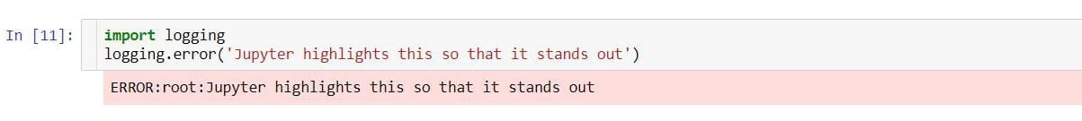
Configuring Logging

Did yous know that Jupyter has a built-in way to prominently display custom error messages in a higher place cell output? This can be handy for ensuring that errors and warnings about things like invalid inputs or parameterisations are difficult to miss for anyone who might exist using your notebooks. An like shooting fish in a barrel, customisable way to hook into this is via the standard Python logging module.

(Note: Merely for this section, nosotros'll use some screenshots and then that we can see how these errors look in a real notebook.)

The logging output is displayed separately from print statements or standard cell output, actualization above all of this.

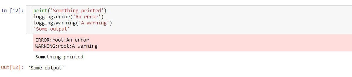
This actually works because Jupyter notebooks listen to both standard output streams, stdout and stderr, merely handle each differently; impress statements and prison cell output route to stdout and by default logging has been configured to stream over stderr.

This means we can configure logging to display other kinds of messages over stderr too.

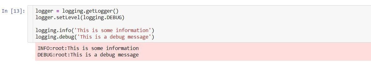
We can customise the format of these messages similar so:

Note that every time yous run a jail cell that adds a new stream handler via logger.addHandler(handler), you volition receive an additional line of output each time for each message logged. We could place all the logging config in its ain prison cell virtually the top of our notebook and leave information technology be or, as we take washed here, animal force supervene upon all existing handlers on the logger. We had to do that in this case anyhow to remove the default handler.

It's besides easy to log to an external file, which might come up in handy if you're executing your notebooks from the command line equally discussed later. Only use a FileHandler instead of a StreamHandler:

<lawmaking="linguistic communication-python">handler = logging.FileHandler(filename='important_log.log', mode='a')</code="language-python">

A final affair to notation is that the logging described hither is not to be confused with using the %config magic to change the awarding's logging level via %config Application.log_level="INFO", as this determines what Jupyter outputs to the terminal while it runs.

Extensions

Every bit it is an open source webapp, plenty of extensions have been adult for Jupyter Notebooks, and there is a long official list. Indeed, in the Working with Databases department below we use the ipython-sql extension. Another of particular note is the package of extensions from Jupyter-contrib, which contains individual extensions for spell check, lawmaking folding and much more.

You can install and prepare this upward from the command line like and so:

<code="linguistic communication-python"> pip install jupyter_contrib_nbextensions jupyter contrib nbextension install --user jupyter nbextension enable spellchecker/primary jupyter nbextension enable codefolding/main </code="language-python">

This will install the jupyter_contrib_nbextensions package in Python, install information technology in Jupyter, and then enable the spell check and code folding extensions. Don't forget to refresh whatsoever notebooks live at the time of installation to load in changes.

Notation that Jupyter-contrib only works in regular Jupyter Notebooks, but there are new extensions for JupyterLab now being released on GitHub.

Enhancing Charts with Seaborn

One of the about common exercises Jupyter Notebook users undertake is producing plots. But Matplotlib, Python's virtually pop charting library, isn't renowned for attractive results despite it's customisability. Seaborn instantly prettifies Matplotlib plots and even adds some additional features pertinent to information science, making your reports prettier and your task easier. It's included in the default Anaconda installation or easily installed via pip install seaborn.

Let'due south check out an example. Offset, we'll import our libraries and load some data.

<code="linguistic communication-python"> import matplotlib.pyplot equally plt import seaborn as sns data = sns.load_dataset("tips") </code="linguistic communication-python">

Seaborn provides some built-in sample datasets for documentation, testing and learning purposes, which we will brand utilise of hither. This "tips" dataset is a pandas DataFrame listing some billing information from a bar or eatery. We can see the size of the total bill, the tip, the gender of the payer, and another attributes.

<code="linguistic communication-python">data.caput()</code="linguistic communication-python">

	total_bill	tip	sex activity	smoker	day	fourth dimension	size
0	16.99	1.01	Female	No	Sun	Dinner	2
ane	x.34	1.66	Male person	No	Sun	Dinner	3
ii	21.01	3.50	Male	No	Sun	Dinner	3
3	23.68	3.31	Male	No	Sun	Dinner	2
4	24.59	3.61	Female	No	Sunday	Dinner	4

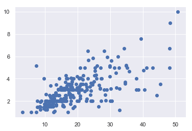
We can easily plot total_bill vs tip in Matplotlib.

<code="language-python">plt.besprinkle(information.total_bill, information.tip);</lawmaking="language-python">

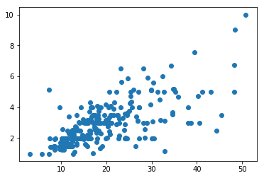
Plotting in Seaborn is just as easy! Simply set a way and your Matplotlib plots will automatically be transformed.

<code="linguistic communication-python">sns.prepare(style="darkgrid")plt.scatter(data.total_bill, data.tip);</code="language-python">

What an improvement, and from only one import and a single extra line! Hither, we used the darkgrid style, but Seaborn has a total of five built-in styles for y'all to play with: darkgrid, whitegrid, dark, white, and ticks.

Merely we don't have to stop with styling: as Seaborn is closely integrated with pandas data structures, its own scatter plot function unlocks additional features.

<code="language-python">sns.scatterplot(ten="total_bill", y="tip", data=data);</code="language-python">

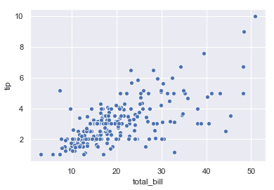
Now we get default centrality labels and an improved default marker for each data betoken. Seaborn tin besides automatically group past categories inside your information to add another dimension to your plots. Let's change the color of our markers based on whether the group paying the nib were smokers or non.

<code="language-python">sns.scatterplot(x="total_bill", y="tip", hue="smoker", information=data);</code="linguistic communication-python">

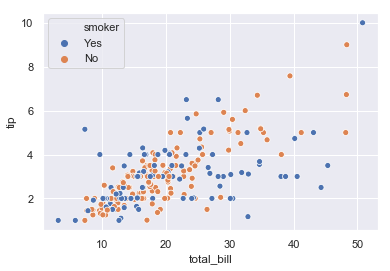
That's pretty neat! In fact, nosotros tin can take this much farther, but there's simply too much detail to go into here. As a taster though, let's colour by the size of the party paying the bill while as well discriminating between smokers and not-smokers.

<code="language-python">sns.scatterplot(10="total_bill", y="tip", hue="size", style="smoker", data=data);</code="language-python">

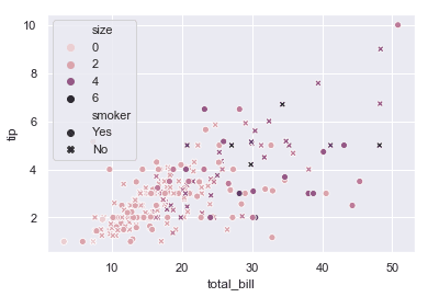
Hopefully it's becoming clear why Seaborn describes itself as a "loftier-level interface for drawing attractive statistical graphics."

Indeed, it'southward high-level plenty to, for example, provide one-liners for plotting data with a line of best fit (determined through linear regression), whereas Matplotlib relies on yous to prepare the information yourself. But if all you lot need is more attractive plots, it's remarkably customisable; for instance, if y'all aren't happy with the default themes, you tin choose from a whole array of standard colour palettes or define your own.

For more means Seaborn allows you to visualise the structure of your data and the statistical relationships within it, bank check out their examples.

Macros

Like many users, you probably observe yourself writing the same few tasks over and over again. Maybe there's a bunch of packages you ever need to import when starting a new notebook, a few statistics that you lot find yourself calculating for every single dataset, or some standard charts that you lot've produced endless times?

Jupyter lets you save code snippets as executable macros for use across all your notebooks. Although executing unknown code isn't necessarily going to be useful for anyone else trying to read or use your notebooks, it'southward definitely a handy productivity boost while you're prototyping, investigating, or just playing around.

Macros are just code, so they can comprise variables that volition have to be defined before execution. Let'southward define one to apply.

<code="language-python">proper noun = 'Tim'</code="language-python">

At present, to ascertain a macro nosotros first need some code to use.

<lawmaking="language-python">impress('Hello, %s!' % name)</code="language-python">

<code="language-python">Hello, Tim!</code="language-python">

We use the %macro and %store magics to fix a macro that's reusable across all our notebooks. It'south mutual to begin macro names with a double underscore to distinguish them from other variables, like so:

<code="linguistic communication-python">%macro -q __hello_world 23 \%shop __hello_world</code="language-python">

<lawmaking="linguistic communication-python">Stored '__hello_world' (Macro)</code="language-python">

The %macro magic takes a name and a cell number (the number in the square brackets to the left of the jail cell; in this case 23 equally in In [23]), and we've also passed -q to arrive less verbose. %store actually allows us to save any variable for utilise in other sessions; hither, we pass the name of the macro nosotros created so we tin can use it again after the kernel is shut downwardly or in other notebooks. Run without any parameters, %store lists your saved items.

To load the macro from the store, we just run:

<lawmaking="language-python">%store -r __hello_world</code="language-python">

And to execute it, nosotros merely demand to run a cell that solely contains the macro proper name.

<code="language-python">__hello_world</lawmaking="linguistic communication-python">

<lawmaking="language-python">Hello, Tim!</code="language-python">

Let's change the variable nosotros used in the macro.

<code="language-python">proper name = 'Ben'</code="linguistic communication-python">

When nosotros run the macro now, our modified value is picked up.

<lawmaking="language-python">__hello_world</lawmaking="language-python">

<code="linguistic communication-python">Hullo, Ben!</lawmaking="language-python">

This works because macros only execute the saved code in the scope of the cell; if proper name was undefined nosotros'd get an fault.

But macros are far from the only way to share code across notebooks.

Executing External Code

Not all code belongs in a Jupyter Notebook. Indeed, while it's entirely possible to write statistical models or fifty-fifty unabridged multi-role projects in Jupyter notebooks, this code becomes messy, difficult to maintain, and unusable by others. Jupyter's flexibility is no substitute for writing well-structured Python modules, which are trivially imported into your notebooks.

In full general, when your quick notebook project starts to get more than serious and you discover yourself writing lawmaking that is reusable or tin be logically grouped into a Python script or module, y'all should practice it! Aside from the fact that you can import your own modules directly in Python, Jupyter also lets you %load and %run external scripts to support better organised, larger-calibration projects and reusability.

Tasks such equally importing the same set of packages over and over for every projection project are a perfect candidate for the %load magic, which will load an external script into the cell in which it'south executed.

But enough talk already, allow's look at an example! If we create a file imports.py containing the following lawmaking:

<code="language-python">  import pandas as pd import numpy as np import matplotlib.pyplot every bit plt</code="language-python">

We tin load this but past writing a one-line code cell, similar so:

<code="linguistic communication-python">%load imports.py</code="language-python">

Executing this will replace the cell contents with the loaded file.

<code="language-python"> # %load imports.py  import pandas every bit pd import numpy equally np import matplotlib.pyplot as plt </code="language-python">

Now we can run the cell once more to import all our modules and we're ready to go.

The %run magic is similar, except information technology will execute the code and display any output, including Matplotlib plots. Y'all tin can even execute entire notebooks this way, merely think that not all code truly belongs in a notebook. Permit'southward check out an example of this magic; consider a file containing the following short script.

<lawmaking="linguistic communication-python"> import numpy as np import matplotlib.pyplot as plt import seaborn as sns sns.set(manner="darkgrid") if __name__ == '__main__': h = plt.hist(np.random.triangular(0, v, 9, yard), bins=100, linewidth=0) plt.show()</code="language-python">

When executed via %run, we get the following consequence.

<code="language-python">%run triangle_hist.py</lawmaking="language-python">

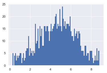
<code="language-python"><matplotlib.effigy.Figure at 0x2ace50fe860></code="linguistic communication-python">

If you wish to laissez passer arguments to a script, merely list them explicitly later on the filename %run my_file.py 0 "Hello, World!" or using variables %run $filename {arg0} {arg1}. Additionally, use the -p option to run the lawmaking through the Python profiler.

Scripted Execution

Although the foremost power of Jupyter Notebooks emanates from their interactive menses, it is besides possible to run notebooks in a not-interactive fashion. Executing notebooks from scripts or the command line provides a powerful mode to produce automated reports or similar documents.

Jupyter offers a control line tool that can be used, in its simplest form, for file conversion and execution. As you are probably aware, notebooks tin be converted to a number of formats, available from the UI under "File > Download As", including HTML, PDF, Python script, and fifty-fifty LaTeX. This functionality is exposed on the command line through an API chosen nbconvert. Information technology is also possible to execute notebooks inside Python scripts, but this is already well documented and the examples below should be equally applicable.

It's of import to stress, similarly to %run, that while the ability to execute notebooks standalone makes information technology possible to write all manor of projects entirely inside Jupyter notebooks, this is no substitute for breaking up code into standard Python modules and scripts equally advisable.

On the Control Line

It will become clear later on how nbconvert empowers developers to create their own automated reporting pipelines, but kickoff allow'due south await at some simple examples. The basic syntax is:

<code="language-python">jupyter nbconvert --to <format> notebook.ipynb</code="language-python">

For example, to create a PDF, simply write:

<code="language-python">jupyter nbconvert --to pdf notebook.ipynb</lawmaking="language-python">

This will take the currently saved static content of notebook.ipynb and create a new file chosen notebook.pdf. One caveat hither is that to convert to PDF requires that you have pandoc (which comes with Anaconda) and LaTeX (which doesn't) installed. Installation instructions depend on your operating system.

By default, nbconvert doesn't execute your notebook code cells. But if you likewise wish to, yous tin can specify the --execute flag.

<code="language-python">jupyter nbconvert --to pdf --execute notebook.ipynb</code="language-python">

A common snag arises from the fact that whatever error encountered running your notebook volition halt execution. Fortunately, you can throw in the --let-errors flag to instruct nbconvert to output the error message into the cell output instead.

<lawmaking="language-python">jupyter nbconvert --to pdf --execute --allow-errors notebook.ipynb</lawmaking="language-python">

Parameterization with Environment Variables

Scripted execution is especially useful for notebooks that don't always produce the aforementioned output, such as if you are processing data that alter over time, either from files on deejay or pulled down via an API. The resulting documents tin easily exist emailed to a list of subscribers or uploaded to Amazon S3 for users to download from your website, for example.

In such cases, it'due south quite likely yous may wish to parameterize your notebooks in society to run them with different initial values. The simplest way to reach this is using environs variables, which you define before executing the notebook.

Let'south say we want to generate several reports for different dates; in the first cell of our notebook, nosotros tin pull this information from an environment variable, which we will proper noun REPORT_DATE. The %env line magic makes it easy to assign the value of an environs variable to a Python variable.

<lawmaking="linguistic communication-python">report_date = %env REPORT_DATE</lawmaking="language-python">

Then, to run the notebook (on UNIX systems) we can do something like this:

<lawmaking="language-python">REPORT_DATE=2018-01-01 jupyter nbconvert --to html --execute report.ipynb</code="language-python">

Equally all environment variables are strings, nosotros will accept to parse them to get the data types we want. For example:

<lawmaking="language-python"> A_STRING="Hello, Tim!" AN_INT=42 A_FLOAT=three.fourteen A_DATE=2017-12-31 jupyter nbconvert --to html --execute example.ipynb</code="language-python">

And nosotros merely parse like and then:

<lawmaking="language-python"> import datetime as dt the_str = %env A_STRING int_str = %env AN_INT my_int = int(int_str) float_str = %env A_FLOAT my_float = float(float_str) date_str = %env A_DATE my_date = dt.datetime.strptime(date_str, '%Y-%thousand-%d') </code="linguistic communication-python">

Parsing dates is definitely less intuitive than other common information types, simply as usual there are several options in Python.

On Windows

If yous'd similar to set your environment variables and run your notebook in a single line on Windows, it isn't quite as unproblematic:

<code="language-python">cmd /C "set A_STRING=Hello, Tim!&& set AN_INT=42 && set A_FLOAT=3.xiv && set up A_DATE=2017-12-31&& jupyter nbconvert --to html --execute example.ipynb"</code="linguistic communication-python">

Nifty readers will discover the lack of a space afterwards defining A_STRING and A_DATE above. This is because trailing spaces are significant to the Windows set command, and so while Python will successfully parse the integer and the float by kickoff stripping whitespace, we take to be more careful with our strings.

Parameterization with Papermill

Using environment variables is fine for simple use-cases, but for anything more than circuitous there are libraries that will allow y'all laissez passer parameters to your notebooks and execute them. With over grand stars on GitHub, probably the most popular is Papermill, which tin can be installed with pip install papermill.

Papermill injects a new cell into your notebook that instantiates the parameters y'all laissez passer in, parsing numeric inputs for you. This means you can simply use the variables without any extra gear up-upward (though dates still need to be parsed). Optionally, you can create a jail cell in your notebook that defines your default parameter values by clicking "View > Jail cell Toolbar > Tags" and calculation a "parameters" tag to the prison cell of your choice.

Our before example that produced an HTML document now becomes:

<code="language-python">papermill example.ipynb example-parameterised.ipynb -p my_string "Hello, Tim!" -p my_int 3 -p my_float iii.1416 -p a_date 2017-12-31 jupyter nbconvert example-parameterised.ipynb --to html --output example.html</lawmaking="language-python">

We specify each parameter with the -p option and employ an intermediary notebook so every bit not to change the original. Information technology is perfectly possible to overwrite the original case.ipynb file, but remember that Papermill will inject a parameter cell.

At present our notebook set-up is much simpler:

<code="language-python"> # my_string, my_int, and my_float are already defined! import datetime equally dt my_date = dt.datetime.strptime(a_date, '%Y-%1000-%d') </lawmaking="language-python">

Our brief glance and so far uncovers simply the tip of the Papermill iceberg. The library can also execute and collect metrics beyond notebooks, summarise collections of notebooks, and it provides an API for storing data and Matplotlib plots for access in other scripts or notebooks. Information technology'southward all well documented in the GitHub readme, and so there's no need to reiterate here.

It should now be clear that, using this technique, it is possible to write trounce or Python scripts that can batch produce multiple documents and be scheduled via tools like crontab to run automatically on a schedule. Powerful stuff!

Styling Notebooks

If you're looking for a particular look-and-feel in your notebooks, y'all can create an external CSS file and load it with Python.

<code="linguistic communication-python"> from IPython.display import HTML HTML('<style>{}</fashion>'.format(open('custom.css').read()))</code="linguistic communication-python">

This works considering IPython'southward HTML objects are inserted straight into the cell output div as raw HTML. In fact, this is equivalent to writing an HTML cell:

<lawmaking="language-python">  <style>.css-instance { color: darkcyan; }</style></code="language-python">

To demonstrate that this works let's use another HTML cell.

<code="linguistic communication-python">%%html <span class='css-example'>This text has a nice colour</bridge></code="language-python">

This text has a nice colour

Using HTML cells would exist fine for i or two lines, only information technology volition typically be cleaner to load an external file every bit we starting time saw.

If yous would rather customise all your notebooks at in one case, you tin can write CSS direct into the ~/.jupyter/custom/custom.css file in your Jupyter config directory instead, though this will only work when running or converting notebooks on your own calculator.

Indeed, all of the aforementioned techniques volition besides piece of work in notebooks converted to HTML, but will not work in converted PDFs.

To explore your styling options, remember that equally Jupyter is just a web app y'all can use your browser's dev tools to inspect it while it's running or delve into some exported HTML output. You will quickly find that information technology is well-structured: all cells are designated with the cell class, text and code cells are likewise respectively demarked with text_cell and code_cell, inputs and outputs are indicated with input and output, and so on.

There are also various dissimilar popular pre-designed themes for Jupyter Notebooks distributed on GitHub. The most pop is jupyterthemes, which is bachelor via pip install jupyterthemes and it'due south as simple as running jt -t monokai to set the "monokai" theme. If yous're looking to theme JupyterLab instead, there is a growing listing of options popping upwardly on GitHub also.

Although it's bad do to hide parts of your notebook that would assistance other people'south agreement, some of your cells may not be important to the reader. For example, you might wish to hide a cell that adds CSS styling to your notebook or, if you wanted to hibernate your default and injected Papermill parameters, y'all could modify your nbconvert call similar so:

<code="language-python">jupyter nbconvert example-parameterised.ipynb --to html --output instance.html --TagRemovePreprocessor.remove_cell_tags="{'parameters', 'injected-parameters'}"</lawmaking="language-python">

In fact, this approach can be applied selectively to any tagged cells in your notebook, making the TagRemovePreprocessor configuration quite powerful. Equally an aside, there are also a host of other ways to hibernate cells in your notebooks.

Working with Databases

Databases are a data scientist's bread and butter, so smoothing the interface between your databases and notebooks is going to exist a real benefaction. Catherine Devlin's IPython SQL magic extension let's you write SQL queries directly into code cells with minimal boilerplate likewise as read the results straight into pandas DataFrames. Commencement, go alee and:

<code="language-python">pip install ipython-sql</lawmaking="linguistic communication-python">

With the package installed, nosotros start things off by executing the following magic in a code cell:

<code="linguistic communication-python">%load_ext sql</lawmaking="linguistic communication-python">

This loads the ipython-sql extension we just installed into our notebook. Let'south connect to a database!

<lawmaking="language-python">%sql sqlite://</code="language-python">

<code="language-python">'Connected: @None'</code="linguistic communication-python">

Here, nosotros just connected to a temporary in-memory database for the convenience of this case, simply you'll probably want to specify details advisable to your database. Connection strings follow the SQLAlchemy standard:

<code="linguistic communication-python">dialect+driver://username:[email protected]:port/database</code="language-python">

Yours might look more similar postgresql://scott:[email protected]/mydatabase, where driver is postgresql, username is scott, password is tiger, host is localhost and the database name is mydatabase.

Note that if yous leave the connectedness string empty, the extension volition endeavor to apply the DATABASE_URL environment variable; read more than about how to customise this in the Scripted Execution section above.

Adjacent, let's rapidly populate our database from the tips dataset from Seaborn nosotros used before.

                      tips = sns.load_dataset("tips") \%sql PERSIST tips                  

<code="language-python"> * sqlite:// 'Persisted tips'</code="language-python">

We can now execute queries on our database. Notation that we tin can use a multiline prison cell magic %% for multiline SQL.

<code="linguistic communication-python">  SELECT * FROM tips LIMIT iii</code="language-python">

<code="language-python"> * sqlite:// Done. </code="language-python">

index	total_bill	tip	sex	smoker	day	time	size
0	16.99	ane.01	Female	No	Sun	Dinner	2
1	10.34	1.66	Male	No	Sun	Dinner	3
ii	21.01	iii.5	Male	No	Sun	Dinner	3

You tin parameterise your queries using locally scoped variables by prefixing them with a colon.

<code="language-python"> meal_time = 'Dinner'  </lawmaking="linguistic communication-python">

<code="language-python"> * sqlite:// Washed. </code="language-python">

index	total_bill	tip	sex	smoker	twenty-four hours	time	size
0	16.99	i.01	Female	No	Lord's day	Dinner	2
1	10.34	1.66	Male person	No	Sun	Dinner	3
2	21.01	3.5	Male	No	Lord's day	Dinner	3

The complexity of our queries is not limited by the extension, and then we can easily write more expressive queries such equally finding all the results with a total pecker greater than the mean.

<code="language-python"> result = %sql SELECT * FROM tips WHERE total_bill > (SELECT AVG(total_bill) FROM tips) larger_bills = consequence.DataFrame() larger_bills.head(3) </code="linguistic communication-python">

<lawmaking="language-python"> * sqlite:// Done. </code="language-python">

	index	total_bill	tip	sexual activity	smoker	day	time	size
0	2	21.01	iii.50	Male	No	Sunday	Dinner	three
ane	three	23.68	iii.31	Male	No	Sun	Dinner	two
2	iv	24.59	three.61	Female	No	Sun	Dinner	4

And every bit you can see, converting to a pandas DataFrame was easy too, which makes plotting results from our queries a piece of block. Allow's bank check out some 95% confidence intervals.

<code="language-python"> sns.lmplot(ten="total_bill", y="tip", hue="smoker", data=larger_bills); </code="language-python">

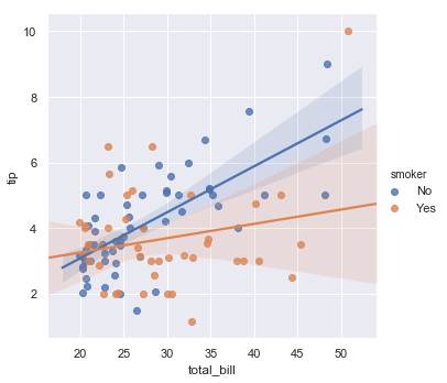
The ipython-sql extension likewise integrates with Matplotlib to let you phone call .plot(), .pie(), and .bar() straight on your query result, and can dump results direct to a CSV file via .csv(filename='my-file.csv'). Read more than on the GitHub readme.

Wrapping Upwards

From the start of the Jupyter Notebooks tutorial for beginners through to here, nosotros've covered a wide range of topics and really laid the foundations for what information technology takes to become a Jupyter master. These manufactures aim serve as a demonstration of the breadth of use-cases for Jupyter Notebooks and how to use them finer. Hopefully, y'all have gained a few insights for your own projects!

There's still a whole host of other things we tin can exercise with Jupyter notebooks that we oasis't covered, such every bit creating interactive controls and charts, or developing your own extensions, but let's leave these for another solar day. Happy coding!

Get Free Data Scientific discipline Resource

Sign upwardly for free to get our weekly newsletter with data science, Python, R, and SQL resource links. Plus, you lot get access to our gratis, interactive online course content!

SIGN UP

starktherens.blogspot.com

Source: https://www.dataquest.io/blog/advanced-jupyter-notebooks-tutorial/

Share this post